Continuous Profiling: The Missing Fourth Pillar of Observability

Observability teams have spent the last decade wiring up metrics, logs, and traces, and most production stacks now have all three running well. Yet incidents still end the same way: the dashboard is green, the trace points to a slow span, and nobody on the call can say why that function is suddenly burning three times the CPU it did last week.

That gap exists because metrics, logs, and traces answer different questions than the one engineers actually need answered during an incident. Metrics show what changed at an aggregate level. Logs show what happened as discrete events. Traces show where time went as a request crossed services. None of them go down to the function or line of code actually responsible for the resource spike, which means teams still fall back on guesswork, redeploys, or a manual profiling session that should have started an hour earlier.

Continuous profiling closes that gap by sampling call stacks in production, all the time, instead of only when someone remembers to run a profiler during an incident. It is no longer a niche practice reserved for performance engineers. According to CNCF’s 2025 Annual Cloud Native Survey, nearly 20 percent of organizations now run profiling as part of their observability stack, up from a rounding error just a few years back, driven largely by teams needing code-level cost attribution as Kubernetes bills grew harder to explain.

This article covers what continuous profiling actually measures, where OpenTelemetry’s profiling signal stands today, which tools are worth knowing, and how to start rolling it out.

What Is Continuous Profiling?

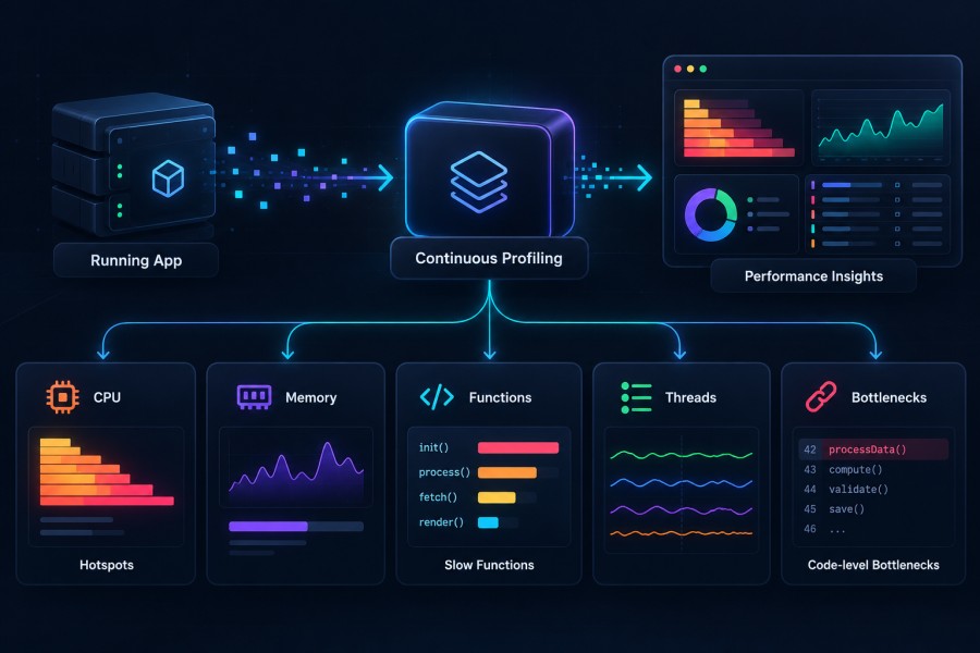
Continuous profiling is the practice of sampling an application’s call stacks in production, at regular intervals, all the time. Instead of asking an engineer to attach a profiler during an incident, the profiler runs quietly in the background and builds a record of exactly where the application spends its CPU cycles, memory, and wait time, every minute of every day.

How it differs from traditional profiling

Traditional profiling was a manual, reactive exercise. An engineer would notice a problem, spin up a local profiler or attach one to a staging environment, reproduce the issue, and dig through the output by hand. That approach works for a known bug in a controlled environment. It falls apart in production, where the conditions that caused a spike often disappear before anyone gets a profiler running.

Continuous profiling flips that order. The data already exists by the time someone needs it, because the profiler never stopped collecting it.

What gets sampled

A continuous profiler typically captures several types of resource data, not just CPU:

• CPU time, to show which functions consume the most processing power
• Memory or heap allocation, to catch leaks and inefficient allocation patterns
• Off-CPU time, to reveal where a thread is blocked waiting on a lock, a network call, or disk I/O
• Goroutine or thread states, particularly useful in Go and Java services under concurrent load

Each of these answers a slightly different question, which is why mature profiling setups rarely rely on CPU sampling alone.

How the data becomes usable

Raw stack samples are not readable on their own. The profiler symbolizes them, mapping machine-level addresses back to function and line numbers, then aggregates thousands of samples into a flame graph. The width of each block in a flame graph represents how much time or resource that function consumed relative to the whole. A wide block near the top of the graph is usually the first place worth looking during a performance investigation.

Why Continuous Profiling Matters Now

Infrastructure metrics tell you a pod is running hot. They do not tell you which function inside that pod is responsible, and that gap has become expensive to ignore.

Kubernetes fragmented resource visibility

A monolith on a handful of servers made resource usage easy to reason about. A fleet of hundreds of short-lived containers does not. Each pod gets rescheduled, resized, and replaced constantly, so infrastructure-level CPU and memory graphs only ever show aggregate noise. Profiling is the only signal that survives that churn, because it attributes resource use to a function, not to a pod that no longer exists an hour later.

This matters more in autoscaled environments than most teams realize. When a horizontal pod autoscaler adds replicas in response to CPU pressure, it is treating the symptom, not the cause. The cluster gets bigger, and the bill gets bigger with it, while the actual function driving that CPU pressure stays invisible unless something is sampling stacks directly.

Cloud cost became an engineering metric

Cloud bills used to be a finance conversation. They are now something engineering leadership gets measured on directly. FinOps teams ask for cost attribution down to the service, and increasingly down to the function, not just the account or the cluster. Infrastructure metrics cannot answer that question. A CPU profile broken down by function can, and it holds up in a cost review in a way a vague utilization graph never will.

Adoption follows where the pressure is sharpest

According to Grafana’s Observability Survey 2025, 18 percent of retail and e-commerce companies report using profiling, compared to just 9 percent in automotive and manufacturing. Retail runs on thin margins per transaction and enormous request volume, so a few percentage points of CPU waste per request compounds fast across billions of requests. That is precisely the kind of waste a flame graph exposes in minutes, where a dashboard only ever shows a slow upward trend.

The same survey found that companies now run an average of eight separate observability technologies, down slightly from the year before, as teams try to consolidate tooling rather than add to it. Profiling is one of the few additions that keeps making the cut, because it replaces a manual, ad hoc process rather than adding a redundant one.

Where teams feel it

A few situations come up often enough that most backend teams will recognize them immediately.

• A deploy goes out, and latency creeps up by a few hundred milliseconds. The trace shows the same span taking longer, but every metric on the service dashboard looks normal, since nothing crossed an alerting threshold. A profile pulled from before and after the deploy usually points straight to the function that regressed, often something as specific as a serialization step or a newly added loop that was not there in the previous build.
• A service’s memory footprint grows steadily over several days until it gets OOM killed and restarted, quietly, without anyone noticing until the third or fourth restart shows up in a weekly review. Heap profiling over that window shows which allocation is never released, long before the crash happens, which turns a recurring mystery into a one-line fix.
• Finance asks why one service costs noticeably more to run than its peers doing similar work. A function-level CPU profile gives an answer that holds up in that conversation, instead of a guess about instance sizing or traffic patterns that may not actually be the cause.
• A team ships a fix for a performance issue everyone agreed was a problem and wants proof it worked before closing the ticket. Comparing profiles from before and after the change shows whether resource use actually dropped, or whether the fix just moved the cost somewhere else in the same request path, which happens more often than most teams expect.

The OpenTelemetry Profiling Signal: Where Things Actually Stand

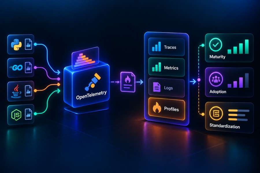
Profiling is the newest signal in OpenTelemetry, and it is still finding its footing. Anyone evaluating it for production needs to know exactly how mature it is before betting a workflow on it.

Profiling arrived last, and later than the rest

OpenTelemetry stabilized traces, metrics, and logs over several years before profiling entered the picture. The project reached CNCF Graduated status in May 2026, and its profiling signal moved into public alpha around the same time, well behind the other three signals in maturity, as OpenTelemetry contributor Dotan Horovits detailed shortly after.

That sequencing matters. Traces, metrics, and logs went through years of production hardening before teams trusted them at scale. Profiling has not had that runway yet, and treating it as equally battle-tested would be a mistake.

Elastic’s contribution shaped the early design

Elastic donated its Universal Profiling agent into the OpenTelemetry profiling effort in 2024, giving the project a working eBPF-based foundation instead of starting from scratch, as The New Stack reported at the time. That donation is a big part of why the profiling signal moved as fast as it did toward public alpha.

What OTLP for profiles actually unlocks

Once profiling speaks the same protocol as traces, metrics, and logs, a CPU spike in a metric can be linked directly to the trace span it occurred in, and from there straight to the function responsible. Today that correlation usually requires stitching together a separate profiling tool with a separate trace backend by hand, matching timestamps and service names manually across two different UIs. A shared protocol removes that manual step entirely, since the profile, the trace, and the metric all carry the same resource attributes from the moment they are collected.

Treat it as alpha, not GA

Schemas and APIs in the profiling signal are still expected to change before general availability. Teams adopting it now should expect to update collector configs and instrumentation as the spec evolves, the same way early adopters of OTel tracing did years ago. The practical move here is to pilot profiling on a single, well-understood service, watch how the signal evolves over the next few release cycles, and expand once the schema settles rather than committing a whole fleet to a spec that is still being finalized.

The Continuous Profiling Tooling

The tooling around continuous profiling splits cleanly into two camps: open source projects built around eBPF or lightweight agents, and profiling features bundled into existing commercial observability platforms. Both are worth knowing before picking a starting point.

Open source options

• Pyroscope: Built by Grafana Labs, it’s the most widely adopted open source continuous profiler. It supports a broad range of languages, including Go, Java, Python, Ruby, and .NET. It slots naturally into a stack already running Grafana, Mimir, or Tempo, since profiles show up alongside the metrics and traces the team already checks daily
• Parca: It’s built by Polar Signals and takes a different approach. It relies on eBPF to sample stacks at the kernel level; a single Parca agent running as a daemonset can profile every process on a node, regardless of language. It’s a strong fit for polyglot environments, where instrumenting every service individually is not realistic. 

eBPF-based agents in general

Beyond Parca specifically, eBPF has become the dominant mechanism for low-overhead, code-free profiling. Because sampling happens in the kernel rather than inside the application process, these agents typically add somewhere between 1 and 5 percent overhead, low enough to run continuously in production without engineering teams needing to negotiate for a maintenance window. 

The tradeoff is that eBPF-based profilers usually need a reasonably recent kernel version and appropriate permissions to load programs into it, which is worth checking against your node images before committing to one, particularly on managed Kubernetes offerings with locked-down node configurations.

Commercial and platform native options

Several established observability vendors have built profiling directly into their existing platforms rather than treating it as a separate product.

• Datadog Continuous Profiler integrates with Datadog’s existing APM and infrastructure monitoring, useful for teams already standardized on Datadog who want profiling in the same UI they already use daily, without adding a separate vendor relationship
• Elastic Universal Profiling ties profiling data to Elastic’s broader search-driven investigation workflow inside Kibana, though it is worth knowing it currently supports CPU profiling only, without memory or off-CPU profiling yet
• AWS CodeGuru Profiler focuses specifically on Java, other JVM languages, and Python, and connects natively to CloudWatch, which makes it a reasonable default for teams already deep in the AWS ecosystem and looking to avoid standing up a separate profiling stack

This is a fast-moving space, and feature sets and pricing change often enough that it is worth checking each vendor’s own documentation directly before making a decision, rather than relying on a comparison written months earlier.

How Continuous Profiling Fits an OTel-Native Stack

Where profiling ends up living in your stack depends on what the rest of the stack is already built on. Platforms architected around OpenTelemetry from the start are in a different position than ones bolting OTLP support onto an older, proprietary agent.

What OTel-native architecture looks like today

CubeAPM ingests traces, metrics, and logs natively over OTLP, rather than converting them from a proprietary agent format. That is the current state of the platform, and it is worth understanding because it shapes what adopting a fourth signal looks like later.

Why architecture matters more than feature lists

Profiling is still moving through OpenTelemetry’s alpha stage, and no platform’s current feature set should be judged against a signal that is not GA yet. What is worth evaluating now is how much rework a future profiling rollout would take on the platform you pick:

• On an OTel-native pipeline, a new signal is largely a config and collector update
• On a proprietary agent, adopting profiling later usually means a second tool, second UI, and second pipeline

Two teams, one year from now

Picture two teams running the same microservices fleet, both deciding a year from now that they need profiling.

• Team one is on a platform built around a proprietary agent for traces and metrics. Adding profiling means evaluating a separate profiling product, standing up a second agent alongside the one already running, and building a manual bridge between two UIs to correlate a profile with the trace that triggered the investigation
• Team two is on an OTel-native platform, where the collector already speaks OTLP for every signal it handles. Adding profiling means updating the collector config to accept the new signal type and pointing it at the same backend everything else already flows into

The engineering effort is not comparable, and team two gets correlated data on day one instead of after weeks of integration work.

What to actually ask a vendor

A few direct questions separate genuine OTel-native architecture from a proprietary platform with an OTLP ingestion endpoint bolted on for compatibility:

• Is OTLP the primary data format the platform stores and queries against, or is it converted into a proprietary internal format on ingest?
• When OpenTelemetry adds a new signal type, does the vendor’s own roadmap show a plan to support it, or has the vendor stayed silent on it?
• Can existing traces and metrics already be queried and correlated together today, which is a reasonable proxy for how well a fourth signal will correlate once it arrives?

Getting Started: A Practical Adoption Path

Rolling out continuous profiling fleet-wide on day one is the most common way teams end up abandoning it within a quarter. A narrower start works better and gets useful results faster.

Step 1: Start with one service

Pick a service that is either expensive to run or has a history of unexplained performance regressions. That gives the team a concrete question to answer, rather than a pile of flame graphs with no clear starting point. Expanding to more services is easy once the first one proves the workflow is worth the effort.

Step 2: Begin with CPU profiling

CPU profiles are the easiest to read and the fastest to act on, which makes them the right entry point. Add memory and off-CPU profiling once the team is comfortable reading a flame graph under pressure during an actual incident.

Step 3: Correlate against existing traces and metrics early

Profiling data is most useful next to the traces and metrics a team already trusts. Set up that correlation before expanding profiling to more services, so the workflow from alert to trace to profile is already proven on one service before it needs to scale.

Step 4: Set a review cadence

Profiling data that only gets opened during an outage misses most of its value. A short weekly review of flame graphs for the most expensive services tends to catch slow regressions long before they become incidents worth paging anyone for.

What a first month of piloting actually looks like

Breaking the rollout into weeks helps set expectations for how fast this moves in practice:

• Week 1: Deploy the profiler on the chosen service, confirm data is flowing, and let it collect a baseline with no analysis yet
• Week 2: Pull the first flame graphs, walk through them as a team, and identify one or two functions worth investigating
• Week 3: Correlate the profile against existing traces for the same service to confirm the workflow end to end
• Week 4: Hold the first scheduled review and decide whether to expand profiling to a second service

Common pitfalls to avoid

• Profiling every service at once before anyone on the team knows how to read the output
• Underestimating symbolization overhead in interpreted languages like Python and Ruby, where it can be higher than in compiled languages
• Assuming flame graphs are self-explanatory. They are not, and skipping team training on how to read one is the fastest way to make an expensive tool sit unused

Conclusion

Continuous profiling does not replace metrics, logs, or traces. It answers the one question the other three were never built to answer: which line of code is actually responsible for the resource a service is burning right now.

That question used to require a manual profiling session, usually started too late to catch the thing that caused it. Continuous profiling removes that delay by running quietly in the background, so the data is already there by the time anyone needs it.

Adoption is still early, and OpenTelemetry’s profiling signal is still working through its own growing pains. But the direction is clear. As it matures toward general availability, the barrier drops from buying a specialized tool to turning on a fourth signal in a stack teams already run.

If your team is already standardized on OpenTelemetry for traces, metrics, and logs, it is worth taking stock of how that stack is built before profiling becomes something you need. CubeAPM runs natively on OTLP today, which is a reasonable place to start that evaluation.

FAQs

Disclaimer: This article reflects the state of continuous profiling tooling and OpenTelemetry’s profiling signal as of the publish date. Both are evolving, and the profiling signal itself is still in public alpha. Verify current features, language support, and pricing on each vendor’s official documentation before making an adoption decision.